Introduction to Policy Evaluation and Causal Inference

Why Every Evaluation Needs a Counterfactual

Fei Huang, UNSW Sydney

• This chapter sets up the rest of the notes: what policy evaluation is, why it is hard, and how each method in these notes solves the same core problem in a different way.
• The running example is health insurance and mortality, a question where naive comparisons give the wrong sign.
• We finish with a roadmap of the methods and how to choose between them.

Why Policy Evaluation

Policies Rest on Causal Claims

Every Policy Embeds a Causal Claim

• Expanding public health insurance will reduce deaths among low-income adults
• Giving workers a generative AI assistant will raise productivity
• Subsidizing insurance premiums will increase take-up
• Higher credit limits will increase borrowing and stimulate spending

Each claim is about what would happen with the policy compared with what would happen without it.

What Policy Evaluation Asks

1. Did it work? Is there an effect at all?
2. How much? Is the effect large enough to matter relative to cost?
3. For whom? Who gains, who loses, and who is unaffected?
4. Why? Through which mechanism?
5. Would it work elsewhere? At a larger scale, in another country, for another population?

Three Kinds of Questions

Data Can Answer Different Questions

Type	Example (insurance)	What it needs
Description	What share of adults have no health insurance?	Good measurement and sampling
Prediction	Which policyholders are likely to lodge a claim next year?	Patterns that hold in new data
Causation	Would a premium subsidy make uninsured people buy cover?	A counterfactual: what happens with vs. without the subsidy

Prediction Is Not Causation

A model can predict claims very well using variables that do not cause claims (postcode, car colour, the time of day a quote is requested). Machine learning models and LLMs are excellent prediction engines. A policy question, however, asks what would happen if we changed something. That is a causal question, and good prediction does not answer it.

These notes are about causal questions.

The Fundamental Problem

Potential Outcomes

Two Outcomes, Only One Observed

For each person i and a treatment D_i \in \{0, 1\} (e.g., having health insurance):

• Y_i(1): the outcome if person i is treated
• Y_i(0): the outcome if person i is not treated
• The causal effect for person i is Y_i(1) - Y_i(0)

We observe only one of the two: Y_i = D_i \, Y_i(1) + (1 - D_i) \, Y_i(0).

The other one, the counterfactual, is missing for everyone. This is the fundamental problem of causal inference (Holland 1986).

The Way Forward: Averages

We cannot learn individual effects, but we can learn average effects, such as the average treatment effect (ATE) E[Y_i(1) - Y_i(0)], if we can find a group whose outcomes stand in for the missing counterfactual. Every method in these notes is a different way of finding that group. Chapter 2 develops the framework formally.

Estimand, Estimator, Estimate

Three Words Worth Keeping Apart

• Estimand: the quantity we want to know, defined with potential outcomes. Example: the average effect of being sent a letter encouraging insurance enrollment on two-year mortality, among previously uninsured adults aged 45–64: E[Y_i(1) - Y_i(0)] in that population, where treatment is receiving the letter
• Estimator: the recipe we apply to data. Example: the difference in mean two-year mortality between people randomly sent and not sent the letter
• Estimate: the number the recipe produces in our sample. Example: a fall of about 0.06 percentage points (Chapter 3)

A design is credible when its estimator recovers the estimand under assumptions we can defend. A precise estimate of the wrong estimand is still wrong.

Why Naive Comparisons Fail

Comparing the Insured with the Uninsured

The naive comparison of mortality between insured and uninsured people decomposes into two terms:

\underbrace{E[Y_i \mid D_i = 1] - E[Y_i \mid D_i = 0]}_{\text{observed difference}} = \underbrace{E[Y_i(1) - Y_i(0) \mid D_i = 1]}_{\text{effect on the treated}} + \underbrace{E[Y_i(0) \mid D_i = 1] - E[Y_i(0) \mid D_i = 0]}_{\text{selection bias}}

Selection bias is the difference the two groups would have had even without insurance.

• People who expect high medical costs are more likely to buy insurance (adverse selection): selection bias pushes towards insurance looking harmful
• People with higher income and education are more likely to be insured and are healthier anyway: selection bias pushes towards insurance looking helpful

Without a design, we cannot know which force dominates, or by how much.

Simulation: Selection Bias Can Flip the Sign

set.seed(2026)
n <- 100000

# Underlying health risk (higher = sicker); unobserved by the researcher
risk <- rnorm(n)

# Potential outcomes: annual probability of death (in percent)
y0 <- pmax(0, 1.5 + 0.8 * risk)          # without insurance
y1 <- pmax(0, y0 - 0.3)                  # insurance lowers mortality by up to 0.3 pp

# Observational world: sicker people are more likely to buy insurance
d_obs <- rbinom(n, 1, plogis(1.5 * risk))
naive <- mean(ifelse(d_obs == 1, y1, y0)[d_obs == 1]) -
         mean(ifelse(d_obs == 1, y1, y0)[d_obs == 0])

# Experimental world: a coin flip decides who is insured
d_rct <- rbinom(n, 1, 0.5)
y_rct <- ifelse(d_rct == 1, y1, y0)
rct <- mean(y_rct[d_rct == 1]) - mean(y_rct[d_rct == 0])

round(c(true_ATE = mean(y1 - y0), naive_comparison = naive, randomized = rct), 3)

        true_ATE naive_comparison       randomized 
          -0.286            0.536           -0.287 

• The naive comparison says insurance raises mortality, because the insured are sicker to begin with. Randomization removes the selection term and recovers the true protective effect.

Other Ways Correlations Mislead

Six Traps

Trap	Example
Confounding	Firms that adopt AI tools are larger and better managed; their higher productivity is not all due to AI
Reverse causality	Workers who are struggling may be given AI tools because they are struggling
Controlling for a mechanism	Estimating the effect of insurance on health while “controlling for” doctor visits removes the main channel through which insurance works
Reversion to the mean	Drivers selected into a safety program after an unusually bad claims year file fewer claims the next year, program or not
Selection into the sample	Studying only firms that survived a crisis hides the ones the crisis destroyed
Searching and selective reporting	Try enough specifications and some will be “significant” by chance; if only those are published, the literature overstates effects

Internal and External Validity

Two Kinds of Validity

• Internal validity: is the estimate right for the people, place, and time studied?
• External validity: does it carry over to other populations, places, or scales?

Strong designs often buy internal validity with a narrow setting (one firm, one state, units near a cutoff). Keep both in view.

The Evaluation Toolkit

Who Decided Who Was Treated?

The Question That Organizes These Notes

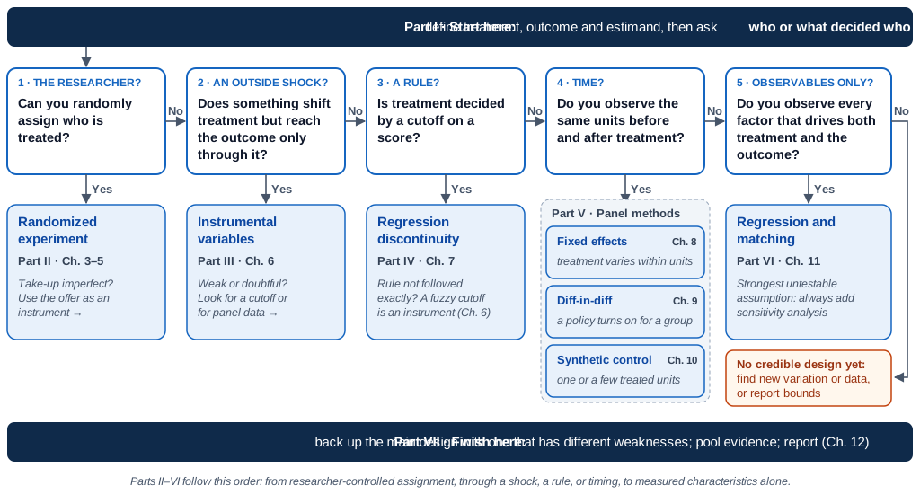
Every method finds a counterfactual by exploiting how treatment was assigned. The notes move from designs where the researcher controls assignment, through designs that exploit a known source of variation (a shock, a rule, timing), to designs that rely only on measured characteristics:

Who or what decided treatment?	Where the counterfactual comes from	Method	Part · Ch.
The researcher	A lottery	Randomized experiment	II · 3–5
An outside shock	Units nudged into treatment by something unrelated to outcomes	Instrumental variables	III · 6
A rule	Units just across a cutoff	Regression discontinuity	IV · 7
The units, observed over time	The same units before treatment, or the change in untreated units	Fixed effects, DiD, synthetic control	V · 8–10
The units, observed once	Similar units, compared on observed characteristics	Regression, matching	VI · 11

Choosing a Design

• Walk through the five questions left to right. Each “no” moves to a design with less control over assignment; the final step relies on the strongest untestable assumption, that every confounder is measured.
• This is a starting point, not a rule. Strong evaluations often combine designs (Chapter 12).

Moving Between Methods

When One Design Runs Into Trouble

Situation	Move to	Why
An experiment where not everyone takes up the treatment	IV (Ch. 5–6)	Random assignment is an instrument for take-up
A cutoff rule that is not followed exactly	Fuzzy RDD = IV at the cutoff (Ch. 6–7)	Crossing the cutoff shifts the probability of treatment
An instrument that is weak or hard to defend, but you have panel data	Fixed effects or DiD (Ch. 8–9)	Use changes within units instead
Treated and comparison groups differ in levels	Fixed effects or DiD (Ch. 8–9)	Fixed differences cancel out
Policy adopted at different times by different units	Heterogeneity-robust DiD (Ch. 9)	Static two-way fixed effects can mislead
Only one or a few treated units, no single good comparison	Synthetic control (Ch. 10)	Build a comparison from a weighted mix
Parallel trends plausible only for similar units	DiD with matching or reweighting (Ch. 9, 11)	Compare like with like, then difference

Methods at a Glance: Designs with Controlled or Quasi-Random Assignment

Method	Key identifying assumption	Main limitation	Ch.
Randomized experiment	Random assignment; no interference	Costly or infeasible; non-compliance, attrition, spillovers	3–5
Instrumental variables	Exclusion restriction; relevance; monotonicity	Untestable exclusion; weak instruments; LATE only	6
Regression discontinuity	Continuity at the cutoff; no manipulation	Effect only at the cutoff	7

Methods at a Glance: Designs Using Time and Observables

Method	Key identifying assumption	Main limitation	Ch.
Panel fixed effects	No time-varying confounders (strict exogeneity)	Time-varying confounders; needs within-unit variation	8
Difference-in-differences	Parallel trends; no anticipation	Trends untestable; staggered-adoption bias in TWFE	9
Synthetic control	Pre-treatment fit carries over	Needs long pre-period; few treated units; placebo inference	10
Regression, matching	No unmeasured confounders; overlap	Blind to unobservables; poor overlap	11

• The full comparison table, with the core idea and estimand for each method, is on the course home page.

The Credibility Revolution

Design Before Estimation

Over the past three decades, empirical economics and management research shifted from “control for everything and hope” to research design: a clear source of variation in treatment that is plausibly as good as random (Angrist and Pischke 2010).

What that means in practice:

• State the comparison that identifies the effect, in plain language
• Make the identifying assumption explicit
• Show evidence for it (balance, pre-trends, placebo tests, first stages)
• Report robustness, and state what the design cannot rule out

How These Notes Work

The Plan of These Notes

Part I: Foundations: what a causal effect is, and how treatment gets assigned

Part II: Randomized Experiments: the researcher assigns treatment; design, practice, and what goes wrong

Part III: Instrumental Variables: an outside shock shifts treatment; from randomized offers to natural instruments

Part IV: Regression Discontinuity: a rule assigns treatment at a cutoff

Part V: Panel Methods: units choose, but we see them over time; fixed effects, DiD, synthetic control

Part VI: Selection on Observables: units choose, and we observe them once; regression and matching

Part VII: Synthesis: combining designs, accumulating evidence, and reporting

LLMs as Research Tools

Measuring Variables with LLMs

LLMs are also increasingly used to measure variables, such as classifying text or rating job tasks. A measured variable is only as good as its validation: measurement error in a treatment variable biases estimates (Chapter 8 shows how fixed effects make this worse).

Six Questions for Any Evaluation

Use These for Any Evaluation You Read or Design

1. Question: What is the causal effect of what, on what, for whom?
2. Estimand: Is the target an ATE, an effect on the treated, or a local effect (compliers, units at a cutoff)?
3. Identification: What comparison identifies the effect, and what assumption makes it valid?
4. Threats: What would break that assumption in this setting?
5. Evidence: How do the authors test or defend the assumption?
6. External validity: Would the result hold in another place, time, or population?

Practicalities

Ethics in Policy Evaluation

Evaluations Involve Real People

• Informed consent and institutional review: ethics board approval, and registration in a public trial registry
• Equipoise: randomizing is easier to justify when we genuinely do not know whether the policy helps, or when resources are limited and must be rationed anyway
• Privacy: linking survey, tax, health, and death records requires secure facilities and disclosure review
• Distribution: average effects can hide harm to specific groups; check heterogeneity
• Complete reporting: pre-registration, pre-analysis plans, and reporting null results

Software and Code

Working with the Code in These Notes

• All examples use R; the packages used are fixest (fixed effects, IV, DiD, event studies), rdrobust and rddensity (regression discontinuity), did (staggered DiD), Synth (synthetic control), and MatchIt (matching)
• Simulations with made-up data and a known true effect show whether each method recovers it; real datasets that ship with these packages (minimum wages, the Basque Country, the LaLonde (1986) job-training data) show the methods at work
• Code is folded by default in both the lecture notes and the slides; click “Code” to expand it

Summary

• Policy evaluation asks what would have happened without the policy
• Individual causal effects are never observed; we estimate averages using a comparison group
• Naive comparisons mix the causal effect with selection bias, which can even flip the sign
• Each method in these notes finds the counterfactual in a different place: chance, an outside shock, a cutoff, time, a synthetic unit, or observed characteristics
• Credible evaluation is about design: a clear comparison, an explicit assumption, and evidence for it

Next Steps

1. Read: Angrist and Pischke (2010); Holland (1986)
2. Practice: In the selection-bias simulation, change the strength of selection (1.5 * risk) to 0 and to −1.5. When is the naive comparison right? When does it overstate the benefit of insurance?
3. Think: Pick one policy you care about. What comparison would identify its effect?
4. Next Class: The potential outcomes framework in detail (Chapter 2)

References

Angrist, Joshua D, and Jörn-Steffen Pischke. 2010. “The Credibility Revolution in Empirical Economics: How Better Research Design Is Taking the Con Out of Econometrics.” Journal of Economic Perspectives 24 (2): 3–30. https://doi.org/10.1257/jep.24.2.3.

Holland, Paul W. 1986. “Statistics and Causal Inference.” Journal of the American Statistical Association 81 (396): 945–60. https://doi.org/10.1080/01621459.1986.10478354.

LaLonde, Robert J. 1986. “Evaluating the Econometric Evaluations of Training Programs with Experimental Data.” American Economic Review 76 (4): 604–20.