Regression Discontinuity Design

When a Rule Decides Treatment at a Cutoff

Fei Huang, UNSW Sydney

• Many policies allocate treatment by a rule: a subsidy for incomes below a threshold, a higher credit limit above a credit score, a scholarship above an exam mark.
• Units just below and just above the threshold are almost identical, except for treatment. Comparing them gives a credible, if local, causal effect.
• Two case studies: subsidized health insurance in Massachusetts (premiums jump at income thresholds), and credit card limits that jump at credit-score cutoffs (a fuzzy design, which links back to IV).

Where This Chapter Fits

Step 3: Is treatment decided by a cutoff on a score?

• You arrive here when: A rule assigns treatment to units above (or below) a threshold on a score, such as income, a test score, or a credit score.
• This chapter: Sharp and fuzzy designs, local linear estimation, bandwidths, and checks for manipulation.
• Next: Chapter 8: when there is no cutoff, but you observe units over time.

See the design flowchart in Chapter 1.

In Practice: Regression Discontinuity

Practitioner Summary

• Use it when: a rule gives treatment to units above (or below) a cutoff on a score
• What you need: the score, the cutoff, the outcome, and many observations close to the cutoff
• What must hold: nothing else changes at the cutoff, and units cannot precisely sort to the favourable side
• Checks to run: a plot of binned means; a density test; smooth covariates; several bandwidths, a donut, and placebo cutoffs; the first stage if the design is fuzzy
• In R: rdrobust(y, x, c = 0) (add fuzzy = d), rdplot(), rddensity()
• Telling a manager: “Households just either side of the threshold are alike except for the subsidy, so the jump at the threshold is the subsidy’s effect for households near it.”

Motivation

Rules with Thresholds Are Everywhere

Treatment Assigned by a Score

Running variable (score)	Cutoff	Treatment
Household income	A share of the poverty line	Larger insurance subsidy
Credit score (FICO)	A lender’s internal cutoff	Higher credit limit
Age	65	Eligibility for public health insurance
Exam score	Admission mark	Selective school place
Firm size	Number of employees	Regulation or reporting rules

The score usually also affects the outcome directly (richer households buy more insurance anyway), so comparing everyone above with everyone below is confounded.

The RDD Idea

Compare Units Just on Either Side

A household at 199% of the poverty line and one at 201% differ in income by very little, but face different subsidies. If nothing else jumps at the cutoff, a jump in the outcome at the cutoff can only come from the jump in treatment.

• The comparison is local: it tells us the effect for units near the cutoff
• In exchange, it requires only that outcomes would have changed smoothly through the cutoff without the treatment

The Sharp Design

Setup and Estimand

Sharp RDD

• Running variable X_i (the score); cutoff c
• Treatment is fully determined by the score: D_i = \mathbb{1}[X_i \geq c] (or X_i < c, as for an income test)
• Estimand: the effect at the cutoff (written here with treatment above the cutoff; reverse the sign when treatment is below it)

\tau_{RD} = \lim_{x \downarrow c} E[Y_i \mid X_i = x] - \lim_{x \uparrow c} E[Y_i \mid X_i = x] = E[Y_i(1) - Y_i(0) \mid X_i = c]

The Key Assumption: Continuity

E[Y_i(0) \mid X_i = x] and E[Y_i(1) \mid X_i = x] are continuous at x = c: without the treatment, average outcomes would not jump at the cutoff.

This fails if units can precisely manipulate their score to land on the preferred side, or if another policy changes at the same cutoff.

Estimation: Local Linear Regression

Fit a Line on Each Side, Near the Cutoff

Within a bandwidth h of the cutoff, regress Y on X - c separately on each side (or with an interaction), usually weighting observations closer to the cutoff more heavily (a triangular kernel). The estimate is the gap between the two fitted lines at X = c.

• Bandwidth trade-off: a narrow window reduces bias (units are more similar) but increases noise
• Data-driven bandwidths choose h to balance the two (Imbens and Kalyanaraman 2012); robust bias-corrected confidence intervals account for the approximation error (Calonico et al. 2014)
• Avoid high-order global polynomials fitted to all the data: they can produce misleading jumps (Gelman and Imbens 2019)
• Software: rdrobust (estimation), rddensity (manipulation tests), rdplot (graphs)

Simulation: A Sharp RDD

suppressMessages({library(rdrobust); library(rddensity)})
set.seed(2026)
n <- 5000

# Income relative to a subsidy cutoff (in % of the poverty line); subsidy below the cutoff
x <- runif(n, -100, 100)
d <- as.integer(x < 0)
# Take-up rises with income anyway, and the subsidy adds 8 points
y <- 40 + 0.15 * x - 0.0008 * x^2 + 8 * d + rnorm(n, 0, 6)

naive <- mean(y[d == 1]) - mean(y[d == 0])
rd <- rdrobust(y, x, c = 0)           # estimates right side minus left side
round(c(naive_comparison = naive,
        RD_effect = -rd$coef[1],      # subsidy is on the left, so flip the sign
        robust_CI_low = -rd$ci[3, 2], robust_CI_high = -rd$ci[3, 1],
        bandwidth = rd$bws[1, 1]), 2)

naive_comparison        RD_effect    robust_CI_low   robust_CI_high 
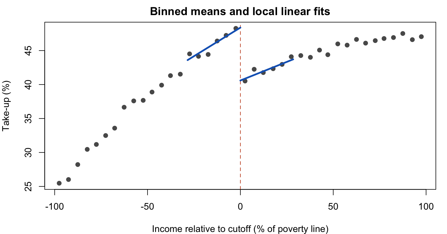
           -7.02             8.10             6.57             9.71 
       bandwidth 
           28.42 

• The naive comparison of eligible and ineligible households even has the wrong sign: richer households buy more insurance regardless of the subsidy.
• RDD compares households near the cutoff and recovers the true 8-point effect.

Seeing the Discontinuity

bins <- cut(x, breaks = seq(-100, 100, by = 5))
bx <- tapply(x, bins, mean); by <- tapply(y, bins, mean)
par(mar = c(4, 4, 2, 1))
plot(bx, by, pch = 19, col = "grey35", xlab = "Income relative to cutoff (% of poverty line)",
     ylab = "Take-up (%)", main = "Binned means and local linear fits")
left <- x < 0 & x > -rd$bws[1, 1]; right <- x >= 0 & x < rd$bws[1, 1]
abline(v = 0, col = "#c2410c", lty = 2)
fl <- lm(y ~ x, subset = left); fr <- lm(y ~ x, subset = right)
lines(c(-rd$bws[1, 1], 0), predict(fl, data.frame(x = c(-rd$bws[1, 1], 0))), lwd = 3, col = "#1565c0")
lines(c(0, rd$bws[1, 1]), predict(fr, data.frame(x = c(0, rd$bws[1, 1]))), lwd = 3, col = "#1565c0")

The Fuzzy Design

When the Rule Is Not Followed Exactly

Fuzzy RDD

Crossing the cutoff changes the probability or amount of treatment, but does not determine it: some units below get treated, some above do not, or the treatment is continuous (a credit limit).

\tau_{FRD} = \frac{\lim_{x \downarrow c} E[Y \mid X = x] - \lim_{x \uparrow c} E[Y \mid X = x]}{\lim_{x \downarrow c} E[D \mid X = x] - \lim_{x \uparrow c} E[D \mid X = x]} = \frac{\text{jump in outcome}}{\text{jump in treatment}}

• This is an instrumental variables estimator (Chapter 6), with “being above the cutoff” as the instrument, used only near the cutoff
• It estimates a LATE for compliers at the cutoff: units whose treatment changes because they cross it
• Needs the IV assumptions locally: the cutoff affects outcomes only through treatment, and monotonicity

Simulation: A Fuzzy RDD

# Credit score relative to a lender's cutoff; the credit limit jumps by about $1,500 above it
fico   <- runif(n, -50, 50)
above  <- as.integer(fico >= 0)
limit  <- 3000 + 20 * fico + 1500 * above + rnorm(n, 0, 400)
borrow <- 1000 + 10 * fico + 0.30 * limit + rnorm(n, 0, 500)   # 30 cents borrowed per extra $1 of limit

fz <- rdrobust(borrow, fico, c = 0, fuzzy = limit)
round(c(estimate = fz$coef[1], robust_CI_low = fz$ci[3, 1], robust_CI_high = fz$ci[3, 2]), 3)

      estimate  robust_CI_low robust_CI_high 
         0.338          0.272          0.422 

Checking the Design

Threats and Diagnostics

What Can Break an RDD

Threat	Diagnostic
Manipulation: units sort precisely to the favourable side	Density test: is there a spike in the number of units just on one side? (McCrary 2008; Cattaneo et al. 2020)
Other differences at the cutoff	Covariate continuity: predetermined characteristics should not jump
Another policy uses the same cutoff	Institutional knowledge; drop that cutoff as a check
Spurious jumps	Placebo cutoffs where nothing changes should show no effect
Sensitivity to choices	Report results for several bandwidths, and a donut that drops units right at the cutoff

Manipulation Test in R

dens <- rddensity(x, c = 0)
c(density_test_p_value = round(dens$test$p_jk, 3))

density_test_p_value 
               0.249 

• A large p-value means no evidence that units bunch on one side. In the simulation, incomes were drawn without manipulation, so the test should not reject.
• In real data, think about who controls the score: households can sometimes adjust reported income; it is much harder for consumers to fine-tune a credit score to land just above a particular lender’s cutoff.

Case Study 1: Subsidized Health Insurance

Case Study 1: How Much Will People Pay for Insurance?

Finkelstein, Hendren & Shepard (2019), American Economic Review (Finkelstein et al. 2019)

Question: How much are low-income adults willing to pay for health insurance, and what does that imply for subsidy design?

Setting: Massachusetts’ subsidized insurance exchange (CommCare), 2009–2013, for adults below 300% of the federal poverty line (FPL) without access to other coverage.

The rule: subsidies fall in steps at 150%, 200%, and 250% of FPL. At each threshold the monthly premium an enrollee pays jumps by about $40, while the plans on offer stay largely the same.

Data: administrative enrollment and claims records, plus survey data to count the eligible population at each income level.

Case Study 1: The Design

Three Discontinuities in Price

• Running variable: income as a percentage of FPL; treatment: the premium an enrollee faces
• Outcomes: take-up of insurance, and the medical costs of those who enroll
• Estimation: linear fits in income on each side of each threshold (a bandwidth of 50% of FPL), with robustness to a 25% bandwidth and quadratic fits
• Demand and cost curves: each threshold gives a price change and a change in who enrolls, tracing out willingness to pay and the costs of marginal enrollees

Case Study 1: Results

Main Findings

• Take-up falls by about 25% (20–24 percentage points) for each $40 increase in the monthly premium: demand is very price-sensitive
• People who drop out when prices rise are cheaper to insure: evidence of adverse selection
• Across the range observed, enrollees’ willingness to pay is less than half of the costs they impose on insurers
• Implication: even generous subsidies leave many uninsured. With premiums at 25% of insurers’ average costs, at most half would enrol; at 10%, at least 20% would remain uninsured

Case Study 1: Threats and Checks

Could People Manipulate Their Income?

• Density checks: no bunching of the eligible population at the thresholds in survey data; slight bunching in enrollment data in 2012–13 has an administrative explanation, and none appears in the base year
• Why manipulation is hard here: applicants reported income, but the formula translating it into subsidy brackets was largely hidden from them, and proof of income was required
• Another change at 200% FPL: at that threshold some groups also lose Medicaid eligibility and copayments rise slightly. Results are robust to dropping that threshold

Case Study 1: What to Copy

Practices to Reuse

• Use every cutoff the rule offers, and drop the one where another policy also changes (200% FPL) as a check.
• Look for bunching in data units cannot influence (survey counts) as well as data they can (enrollment).
• Turn local effects into the curve the decision needs: three price jumps trace out willingness to pay against cost.

Case Study 1: Discussion Questions

1. Why does comparing take-up for everyone above and below 200% FPL not identify the effect of price?
2. What would you expect to see in the data if people misreported income to stay below a threshold?
3. Why is dropping the 200% FPL threshold a useful robustness check?
4. The estimates apply to people near 150%, 200%, and 250% FPL. How far would you extrapolate them?
5. What does “willingness to pay is less than half of expected costs” imply for an insurance mandate?

Case Study 1: Suggested Answers (1–3)

1. Income affects take-up directly: richer households differ in needs, preferences, and access to other coverage. A comparison of everyone above and below mixes the price change with these differences; the RD uses only households close to the threshold.
2. Bunching: more enrollees just below each threshold than just above, and a jump in the density of reported income at the cutoff.
3. At 200% FPL some groups also lose Medicaid eligibility and copayments rise, so more than the premium changes there. Results that hold without that threshold rely only on cutoffs where the premium is the main change.

Case Study 1: Suggested Answers (4–5)

4. Only cautiously. The estimates describe people near 150–250% FPL in Massachusetts’ exchange. The roughly linear patterns between thresholds support modest interpolation within that range, not extrapolation to much poorer or richer people or other markets.
5. Many low-income adults would not buy insurance at its cost even if it were offered at a fair price. Reaching high coverage would need large subsidies or a mandate. One reason the paper discusses is uncompensated care: the uninsured receive some care without paying for it, which lowers the value of insurance to them.

Case Study 2: Credit Limits at Credit-Score Cutoffs

Case Study 2: Do Consumers Borrow More When Banks Lend More?

Agarwal, Chomsisengphet, Mahoney & Stroebel (2018), Quarterly Journal of Economics (Agarwal et al. 2018)

Question: When banks’ cost of funds falls (for example, through monetary policy), does extra credit reach consumers who want to borrow?

Key quantity: the marginal propensity to borrow (MPB): how much extra a consumer borrows for each extra dollar of credit limit.

The rule: banks set credit limits partly by FICO score cutoffs (for example 660, 700, 720, 740, 760). At a cutoff, the credit limit jumps, while consumers just below and just above are otherwise similar.

Case Study 2: The Design

A Fuzzy RDD, Many Times Over

• 743 credit-limit discontinuities across lenders and cutoffs, covering 8.5 million new credit cards within 50 FICO points of a cutoff
• First stage: the credit limit jumps at each cutoff, and the jump persists for years
• Fuzzy RD: the jump in borrowing divided by the jump in credit limit, a local Wald estimator
• Bandwidth: chosen by a data-driven rule for each discontinuity; estimates pooled across discontinuities and by FICO group
• Checks: interest rates, borrower characteristics, and the number of new accounts all move smoothly through the cutoffs

Case Study 2: Results

Main Findings

• The MPB falls with credit score: about 59 cents borrowed per extra dollar of credit limit for consumers with FICO scores below 660, and essentially zero above 740
• For the riskiest borrowers, higher limits reduce banks’ profits, so banks are least willing to lend more to the consumers who most want to borrow
• Policy implication: cheaper funding for banks raises household borrowing only if extra credit reaches low-score consumers, which banks have little incentive to do

Why Credit Scores Are a Good Running Variable

Banks’ credit-limit rules are not known to consumers, and the FICO formula is proprietary, so even a consumer who knew a cutoff would find it very hard to move their score precisely across it (the authors’ argument). Consistent with this, the authors show that the number of new accounts, borrower characteristics, and interest rates all move smoothly through the cutoffs.

Case Study 2: What to Copy

Practices to Reuse

• Pool many discontinuities (743) for precision and to compare groups of borrowers.
• Show the first stage persists before interpreting effects on borrowing.
• Report the parameter policymakers use: the marginal propensity to borrow, by credit score.

Case Study 2: Discussion Questions

1. Why is this a fuzzy rather than a sharp design? What is the “treatment”?
2. Write the fuzzy RD estimate as an IV estimate. What are the instrument, the first stage, and the reduced form?
3. Who are the compliers at a FICO cutoff, and is their MPB the one a central bank cares about?
4. What could make outcomes jump at a FICO cutoff other than the credit limit? How do the authors check?
5. Why does having 743 discontinuities, rather than one, strengthen the conclusions?

Case Study 2: Suggested Answers (1–2)

1. Crossing the cutoff raises the average credit limit, but limits also depend on other factors and vary within each side. The treatment is the credit limit, a continuous amount, so the jump in borrowing is scaled by the jump in the limit.
2. Instrument: an indicator for being above the cutoff. First stage: the jump in the credit limit at the cutoff. Reduced form: the jump in borrowing. The MPB is the reduced form divided by the first stage, estimated near the cutoff.

Case Study 2: Suggested Answers (3–4)

3. New cardholders near a lender’s cutoff whose limit is set by that rule. Central banks care about households whose credit changes when banks’ funding costs change; these borrowers are a relevant group, but local to particular scores and lenders.
4. Other loan terms (interest rates, fees), or banks approving more accounts above the cutoff, which would change who is in the sample. The authors show interest rates, borrower characteristics, and the number of accounts are smooth through the cutoffs.

Case Study 2: Suggested Answers (5)

5. Many cutoffs give precision and let the authors estimate effects across the score distribution. A single cutoff could coincide with some other rule; consistent results across many lenders and cutoffs make that explanation unlikely.

Comparing the Two Designs

Two Applications Compared

Sharp-Style and Fuzzy Designs

	Finkelstein, Hendren & Shepard (2019)	Agarwal et al. (2018)
Running variable	Income (% of poverty line)	Credit score
What jumps	Enrollee premium (about $40)	Credit limit
Design	Price discontinuities used to trace demand and cost	Fuzzy RD (local Wald)
Number of cutoffs	3	743
Manipulation risk	Income reporting; checked with densities	Low: smooth account density and characteristics
Main caveat	Another policy change at 200% FPL	Effects are local to each cutoff

Best Practices

RDD Checklist

Before and After Estimating

1. Know the rule: who sets the cutoff, who controls the score, and whether anything else changes at the cutoff
2. Plot the data: binned means of outcome and treatment against the running variable
3. Estimate locally: local linear regression with a data-driven bandwidth and robust confidence intervals
4. Test for manipulation (density) and covariate continuity
5. Vary the bandwidth, try a donut, and run placebo cutoffs
6. For fuzzy designs, report the first stage and interpret the estimate as a LATE at the cutoff

Common Pitfalls

Mistakes to Avoid

• Fitting high-order polynomials to the whole range of the running variable
• Ignoring manipulation when units can influence their score
• Missing other policies that use the same cutoff
• Treating a local effect at the cutoff as an average effect for everyone
• Using a bandwidth so wide that units far from the cutoff drive the estimate
• Analysing a fuzzy design as if it were sharp

Summary

• When a rule assigns treatment at a cutoff, units just either side form a credible comparison
• The key assumption is continuity: nothing else jumps at the cutoff
• Estimate with local linear regression and data-driven bandwidths; show the plot
• A fuzzy cutoff is an instrument at the threshold, giving a LATE for compliers there
• Manipulation, other policies at the cutoff, and locality are the main concerns

Next Steps

1. Read: Finkelstein et al. (2019) Sections I–II; Agarwal et al. (2018) Sections II–IV; Lee and Lemieux (2010) for a broad review
2. Practice: In the sharp simulation, add manipulation: move 30% of households just above the cutoff to just below. Run rddensity again. What happens to the RD estimate?
3. Next Class: Panel data and fixed effects, when there is no cutoff but units are observed over time (Chapter 8)

References

Agarwal, Sumit, Souphala Chomsisengphet, Neale Mahoney, and Johannes Stroebel. 2018. “Do Banks Pass Through Credit Expansions to Consumers Who Want to Borrow?” The Quarterly Journal of Economics 133 (1): 129–90. https://doi.org/10.1093/qje/qjx027.

Calonico, Sebastian, Matias D Cattaneo, and Rocio Titiunik. 2014. “Robust Nonparametric Confidence Intervals for Regression-Discontinuity Designs.” Econometrica 82 (6): 2295–326. https://doi.org/10.3982/ECTA11757.

Cattaneo, Matias D, Michael Jansson, and Xinwei Ma. 2020. “Simple Local Polynomial Density Estimators.” Journal of the American Statistical Association 115 (531): 1449–55. https://doi.org/10.1080/01621459.2019.1635480.

Finkelstein, Amy, Nathaniel Hendren, and Mark Shepard. 2019. “Subsidizing Health Insurance for Low-Income Adults: Evidence from Massachusetts.” American Economic Review 109 (4): 1530–67. https://doi.org/10.1257/aer.20171455.

Gelman, Andrew, and Guido Imbens. 2019. “Why High-Order Polynomials Should Not Be Used in Regression Discontinuity Designs.” Journal of Business & Economic Statistics 37 (3): 447–56. https://doi.org/10.1080/07350015.2017.1366909.

Imbens, Guido, and Karthik Kalyanaraman. 2012. “Optimal Bandwidth Choice for the Regression Discontinuity Estimator.” Review of Economic Studies 79 (3): 933–59. https://doi.org/10.1093/restud/rdr043.

Lee, David S, and Thomas Lemieux. 2010. “Regression Discontinuity Designs in Economics.” Journal of Economic Literature 48 (2): 281–355. https://doi.org/10.1257/jel.48.2.281.

McCrary, Justin. 2008. “Manipulation of the Running Variable in the Regression Discontinuity Design: A Density Test.” Journal of Econometrics 142 (2): 698–714. https://doi.org/10.1016/j.jeconom.2007.05.005.