Synthetic Control

Building a Comparison When Only One Unit Is Treated

Fei Huang, UNSW Sydney

• Difference-in-differences needs a comparison group whose trend stands in for the treated group’s counterfactual trend. With one treated region, country, or firm, there is often no single unit that does this well.
• Synthetic control builds the comparison: a weighted combination of untreated units chosen to track the treated unit before the intervention.
• Two case studies: the economic cost of terrorism in the Basque Country (the paper that introduced the method), and the stock-market value of connections to Timothy Geithner when he was nominated US Treasury Secretary in 2008.

Where This Chapter Fits

Step 4: Do you observe the same units before and after treatment?

• You arrive here when: Only one or a few units are treated (a country, a state, a firm), and parallel trends with any single comparison group are hard to defend.
• This chapter: Building a comparison unit as a weighted combination of untreated units.
• Next: Chapter 11: when units are observed only once, and we must rely on observed characteristics.

See the design flowchart in Chapter 1.

In Practice: Synthetic Control

Practitioner Summary

• Use it when: one or a few units are treated and no single untreated unit is a convincing comparison
• What you need: the outcome for the treated unit and many untreated units over a long pre-treatment period, plus predictors
• What must hold: the weighted donors would have tracked the treated unit without treatment; no spillovers to donors; no anticipation (or backdate the treatment)
• Checks to run: pre-treatment fit; the weights and predictor balance; in-space and in-time placebos; leave-one-out
• In R: Synth::dataprep() and synth(), tidysynth, synthdid for synthetic DiD
• Telling a manager: “We built a stand-in from regions that tracked ours closely for 15 years. After the event, ours fell about 10% below its stand-in.”

Motivation

When Only One Unit Is Treated

Comparative Case Studies

Many policies and events affect a single large unit:

• A region suffers decades of political violence
• A state passes a tobacco-control law
• A country joins a currency union or leaves a trading bloc
• A firm’s well-connected former adviser becomes a regulator

We observe the treated unit before and after, and many untreated units over the same period.

Why DiD Struggles Here

• Which comparison? Choosing “the most similar region” by hand is subjective and easy to dispute
• The average of all untreated units may follow a very different path from the treated unit, so parallel trends fails
• With one treated unit, the usual standard errors for DiD do not apply

The Method

The Synthetic Control Idea

Choosing the Comparison from the Data

Build a synthetic version of the treated unit as a weighted average of untreated units (the donor pool), with weights chosen so the synthetic unit matches the treated unit before treatment:

• in the path of the outcome over the pre-treatment period, and
• in predictors of the outcome (income, industry mix, population, education)

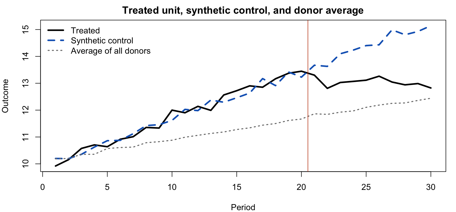
After treatment, the synthetic unit’s outcome is the estimate of what would have happened without treatment. The gap between the two paths is the estimated effect.

The Estimator

Notation

Unit 1 is treated from period T_0 + 1; units 2, \dots, J+1 are never treated.

Weights: W = (w_2, \dots, w_{J+1}) with w_j \geq 0 and \sum_j w_j = 1, chosen to minimize

(X_1 - X_0 W)' \, V \, (X_1 - X_0 W)

where X_1 holds pre-treatment predictors for the treated unit, X_0 the same for donors, and V weights the importance of each predictor.

Effect in each post-treatment period t > T_0:

\hat\tau_t = Y_{1t} - \sum_{j=2}^{J+1} w_j^* \, Y_{jt}

Why Non-Negative Weights That Sum to One?

They prevent extrapolation: the synthetic unit must lie inside the range (the convex hull) of the donors. The method shows plainly when it cannot match the treated unit. If the treated unit is more extreme than every donor on some characteristic, no synthetic control can reproduce it. Even inside that range, averaging very different donors can cause interpolation bias, so the donor pool should be restricted to units similar to the treated one (Abadie 2021).

When Synthetic Control Beats DiD

Allowing for Different Trends

DiD assumes the treated unit and the comparison group would have moved in parallel. Synthetic control allows units to respond differently to common shocks (for example, an industrial region is hit harder by an oil crisis), as long as a weighted mix of donors responds the same way as the treated unit.

A good fit over a long pre-treatment period is the evidence for this: it is unlikely that a mix of donors tracks the treated unit for many years by chance, unless it shares the treated unit’s exposure to the forces driving the outcome (Abadie et al. 2010).

Requirements and Limits

When the Method Is Credible

• Long pre-treatment period with a close fit; a poor fit means the counterfactual is not credible
• Donor pool of units that were not affected by the treatment or by other large shocks in the same period
• No spillovers from the treated unit to donors (otherwise the gap is biased)
• No anticipation: if behaviour changed before the formal treatment date (for example, once a policy was announced), backdate the treatment to that point
• Not too extreme: the treated unit must be within the range of donors on the characteristics that matter
• Inference cannot rely on large-sample standard errors with one treated unit; use placebo tests (Abadie 2021)

Inference

Placebo Tests

Is the Gap Unusual?

In-space placebos: pretend each donor was treated instead, and re-run synthetic control for it (excluding the real treated unit from its donor pool). If the treated unit’s gap is larger than almost all placebo gaps, the effect is unlikely to be chance.

• Compare the ratio of post- to pre-treatment fit error (root mean squared prediction error, RMSPE), which penalizes placebos with poor pre-treatment fit
• p-value = rank of the treated unit’s ratio among all J + 1 units, divided by J + 1. With 20 donors the smallest possible p-value is 1/21 \approx 0.048

In-time placebos: pretend treatment happened at an earlier date. A large “effect” before the real treatment signals a poor design.

Leave-one-out: drop each donor with positive weight in turn; results should not hinge on one donor.

Simulation

Synthetic Control vs. DiD

set.seed(2026)
J <- 20; T0 <- 20; T1 <- 10; TT <- T0 + T1
pre <- 1:T0; post <- (T0 + 1):TT

# Units load differently on a common upward trend (e.g., a growing industry)
lambda <- c(1.8, runif(J, 0, 2))          # unit 1 is treated and strongly exposed
trend  <- seq(0, 3, length.out = TT)
alpha  <- c(10, rnorm(J, 10, 1))
Y <- sapply(1:TT, function(t) alpha + lambda * trend[t] + rnorm(J + 1, 0, 0.15))
effect <- c(rep(0, T0), -seq(0.5, 2.5, length.out = T1))
Y[1, ] <- Y[1, ] + effect                 # true effect: a growing loss

# Weights: non-negative, sum to one (softmax), chosen to fit the pre-period path
sc_weights <- function(y1, Y0) {
  loss <- function(a) { w <- exp(a) / sum(exp(a)); sum((y1 - colSums(w * Y0))^2) }
  a <- optim(rep(0, nrow(Y0)), loss, method = "BFGS", control = list(maxit = 2000))$par
  exp(a) / sum(exp(a))
}
w <- sc_weights(Y[1, pre], Y[-1, pre])
synth <- colSums(w * Y[-1, ])

did <- (mean(Y[1, post]) - mean(Y[1, pre])) -
       (mean(colMeans(Y[-1, post])) - mean(colMeans(Y[-1, pre])))

round(c(true_effect = mean(effect[post]),
        synthetic_control = mean((Y[1, ] - synth)[post]),
        DiD_all_donors = did,
        largest_weight = max(w)), 2)

      true_effect synthetic_control    DiD_all_donors    largest_weight 
            -1.50             -1.39              0.06              0.84 

• The treated unit is more exposed to the common trend than the average donor. DiD against all donors assumes they share the trend, and misses the loss almost entirely.
• Synthetic control puts most weight on the donors with similar exposure and recovers most of the effect.

Seeing the Fit and the Gap

par(mar = c(4, 4, 2, 1))
plot(1:TT, Y[1, ], type = "l", lwd = 3, ylim = range(Y[1, ], synth, colMeans(Y[-1, ])),
     xlab = "Period", ylab = "Outcome", main = "Treated unit, synthetic control, and donor average")
lines(1:TT, synth, lwd = 3, lty = 2, col = "#1565c0")
lines(1:TT, colMeans(Y[-1, ]), lwd = 2, lty = 3, col = "grey50")
abline(v = T0 + 0.5, col = "#c2410c")
legend("topleft", c("Treated", "Synthetic control", "Average of all donors"),
       lty = c(1, 2, 3), lwd = c(3, 3, 2), col = c("black", "#1565c0", "grey50"), bty = "n")

Placebo Inference

# Ratio of post- to pre-treatment RMSPE for every unit, treating it as if treated
rmspe_ratio <- function(i) {
  donors <- setdiff(2:(J + 1), i)          # never use the real treated unit as a donor
  w_i <- sc_weights(Y[i, pre], Y[donors, pre])
  gap <- Y[i, ] - colSums(w_i * Y[donors, ])
  sqrt(mean(gap[post]^2)) / sqrt(mean(gap[pre]^2))
}
ratios <- sapply(1:(J + 1), rmspe_ratio)

c(treated_rank = rank(-ratios)[1],
  units = J + 1,
  p_value = round(rank(-ratios)[1] / (J + 1), 3))

treated_rank        units      p_value 
       1.000       21.000        0.048 

• If the treated unit’s ratio is the largest of all 21, the p-value is 1/21. This is the smallest p-value achievable with 20 donors: synthetic control inference is limited by the size of the donor pool.

Extensions

Beyond the Basic Method

Recent Developments

Extension	Idea
Synthetic DiD (Arkhangelsky et al. 2021)	Combine synthetic-control unit weights with time weights and a DiD comparison; robust when fit is imperfect
Augmented synthetic control (Ben-Michael et al. 2021)	Correct the remaining pre-treatment imbalance with an outcome model
Many treated units	Build a synthetic match for each treated unit, then average (Case Study 2)
Staggered adoption	Units treated at different dates; connects to the robust DiD estimators of Chapter 9

Software: Synth and tidysynth (classic method), synthdid (synthetic DiD), augsynth (augmented).

Real Data

Real Data: Rebuilding the Synthetic Basque Country

suppressMessages(library(Synth))
data(basque)   # Abadie & Gardeazabal's data: 17 Spanish regions (region 17 = Basque Country), 1955-1997

dp <- dataprep(foo = basque, dependent = "gdpcap", unit.variable = "regionno",
  unit.names.variable = "regionname", time.variable = "year",
  treatment.identifier = 17, controls.identifier = c(2:16, 18),   # region 1 is Spain as a whole
  predictors = c("school.illit", "school.prim", "school.med", "school.high", "school.post.high", "invest"),
  predictors.op = "mean", time.predictors.prior = 1964:1969,
  special.predictors = list(list("gdpcap", 1960:1969, "mean"), list("sec.agriculture", seq(1961, 1969, 2), "mean"),
    list("sec.energy", seq(1961, 1969, 2), "mean"), list("sec.industry", seq(1961, 1969, 2), "mean"),
    list("sec.construction", seq(1961, 1969, 2), "mean"), list("sec.services.venta", seq(1961, 1969, 2), "mean"),
    list("sec.services.nonventa", seq(1961, 1969, 2), "mean"), list("popdens", 1969, "mean")),
  time.optimize.ssr = 1960:1969, time.plot = 1955:1997)
invisible(capture.output(so <- synth(dp)))

w <- so$solution.w[, 1]
round(setNames(w, basque$regionname[match(as.numeric(names(w)), basque$regionno)])[w > 0.01], 3)

             Cataluna Madrid (Comunidad De) 
                0.851                 0.149 

• basque ships with the Synth package. The weights reproduce the paper exactly: Catalonia 0.8508, Madrid 0.1492.

Real Data: The Gap

synth_path <- dp$Y0plot %*% so$solution.w
gap_pct <- 100 * (dp$Y1plot - synth_path) / synth_path
par(mar = c(4, 4, 1, 1))
plot(1955:1997, gap_pct, type = "l", lwd = 3, xlab = "Year",
     ylab = "Basque GDP per head vs. synthetic (%)")
abline(h = 0, lty = 2); abline(v = 1975, col = "#c2410c")   # terrorism becomes large-scale

Reading the Result

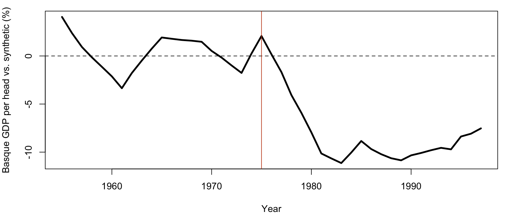
Until the late 1970s the gap stays within a few percent of zero; it then opens to about 8–11% below the synthetic region through the 1980s and 1990s, the paper’s headline result of roughly 10%.

Case Study 1: The Basque Country

Case Study 1: The Economic Cost of Conflict

Abadie & Gardeazabal (2003), American Economic Review (Abadie and Gardeazabal 2003)

Question: What did decades of terrorism cost the economy of the Basque Country?

Context: at the start of ETA’s terrorist campaign in the late 1960s, the Basque Country was the third-richest of Spain’s 17 regions; by the late 1990s it had fallen to sixth. Nearly 800 people were killed, and businesses were targets of extortion and kidnapping.

Why it is hard:

• A before–after comparison mixes terrorism with Spain’s deep recession of the late 1970s and early 1980s
• A comparison with the rest of Spain is misleading: the Basque Country was richer, more industrial, more densely populated, and better educated

Case Study 1: Building the Synthetic Basque Country

Donors, Predictors, and Weights

• Donor pool: the 16 other Spanish regions
• Predictors (1960s): GDP per head, investment ratio, population density, sectoral shares of production, and human capital
• Choice of V: predictor weights chosen so that the synthetic region best reproduces Basque GDP per head in the 1960s
• Result: Catalonia (0.85) and Madrid (0.15); all other regions receive zero weight
• What cannot be matched: the Basque Country had the highest industrial share in Spain, so no weighted average of other regions reproduces it exactly

• Catalonia and Madrid are not surprising: they were the other rich, industrial, densely populated regions. The method makes the choice explicit and reproducible.

Case Study 1: Results

Main Findings

• The Basque Country and its synthetic control track each other closely until about 1975
• Then they diverge as terrorism becomes large-scale: Basque GDP per head falls up to about 12% below the synthetic region, and about 10% on average over the 1980s and 1990s
• The gap tracks terrorist activity: spikes in killings are followed by a widening gap two to three years later
• The Basque population also fell relative to the synthetic region, so the loss in total output was larger still

A Second Test: The 1998–99 Ceasefire

The authors also study stock returns during ETA’s ceasefire. Shares of firms with a large part of their business in the Basque Country outperformed other firms by about 10% as the truce became credible, and underperformed by about 11% when it ended.

Case Study 1: Threats and Checks

Could the Gap Be Something Other Than Terrorism?

• Placebo study: applied to Catalonia (similar, industrial, no comparable terrorism), the method reproduces its GDP path closely until the late 1980s; Catalonia then pulls about 4% ahead of its synthetic control (the 1992 Barcelona Olympics). Because Catalonia is the main donor for the Basque Country, this suggests the Basque gap in the 1990s may be overstated somewhat
• Industrial decline: the Basque Country was more industrial, and industry collapsed after the oil crises. The authors argue this cannot explain why the gap moves with terrorist activity, and controlling for oil prices leaves the link unchanged
• Spillovers to donors: if terrorism also hurt Catalonia or Madrid, the gap understates the effect; if it diverted investment to them, the gap overstates it. The synthetic region’s economy is much larger than the Basque economy, which limits the second concern

Case Study 1: What to Copy

Practices to Reuse

• Fit a long pre-period and show it. Twenty years of close tracking (1955–1975) is what makes the later gap credible.
• Report what you cannot match (the industrial share) instead of hiding it.
• Look for a second, independent test: stock returns during the ceasefire.

Case Study 1: Discussion Questions

1. Why not simply compare the Basque Country with the average of all other Spanish regions?
2. The synthetic control cannot match the Basque industrial share. Why does that matter, and how do the authors respond?
3. Why does the close fit until 1975 make the post-1975 gap more convincing?
4. How does the ceasefire stock-market analysis strengthen the case, given that it uses a completely different design?
5. What spillovers from Basque terrorism to Catalonia could bias the estimate, and in which direction?

Case Study 1: Suggested Answers (1–2)

1. The other regions were on average poorer, less industrial, and less densely populated, and followed different paths before terrorism. Their average is a poor guide to what the Basque economy would have done.
2. The Basque Country was more industrial, and industry declined after the oil crises, so part of the gap could reflect industrial decline. The authors note that the industrial share fell by similar amounts in both (17 vs. 15 points), that the gap follows terrorist activity, and that oil prices do not explain it.

Case Study 1: Suggested Answers (3–4)

3. A weighted mix of regions is unlikely to track the Basque economy for two decades unless it responds to the same economic forces. A long close fit makes it a credible guide to the path without terrorism.
4. It uses different data (share prices) and a different design (an event study around the truce), with different assumptions. Two methods with different weaknesses giving consistent answers are harder to explain away.

Case Study 1: Suggested Answers (5)

5. If terrorism also hurt Catalonia, through fear, trade, or tourism, the synthetic region is lower and the gap understates the effect. If investment moved from the Basque Country to Catalonia, the synthetic region is higher and the gap overstates it.

Case Study 2: Connections in a Crisis

Case Study 2: The Value of Connections to Policymakers

Acemoglu, Johnson, Kermani, Kwak & Mitton (2016), Journal of Financial Economics (Acemoglu et al. 2016)

Question: When policymakers have wide discretion, as in a financial crisis, are firms connected to them worth more?

The event: on 21 November 2008, news leaked that Timothy Geithner, then president of the Federal Reserve Bank of New York, would be nominated US Treasury Secretary.

Treatment: financial firms connected to Geithner, using three alternative measures: meetings on his official schedule in 2007–08, shared board and non-profit memberships, and headquarters in New York City.

Outcome: daily stock returns of financial firms around the announcement.

Case Study 2: The Design

An Event Study, Backed Up by Synthetic Matching

Main approach: abnormal returns relative to a market model estimated over 250 trading days ending 30 days before the event; compare connected and non-connected firms, controlling for size, profitability, and leverage.

The concern: connected firms may differ from non-connected ones in ways that move their returns on the same days.

Synthetic matching: for each connected firm, build a synthetic firm from non-connected financial firms, with weights chosen so the synthetic firm’s daily returns track the connected firm’s returns over the 250-day pre-event window.

• The effect averages each firm’s gap, giving more weight to better matches
• Inference: draw 5,000 placebo treatment groups of the same size from non-connected firms; the real effect is significant if it lies outside the middle 95% of placebo effects

Case Study 2: Results and Checks

Main Findings

• Geithner-connected firms earned a cumulative abnormal return of about 6% after the first full trading day, and about 12% after ten trading days, relative to other financial firms
• When news broke in January 2009 that his confirmation might be derailed by tax issues, connected firms had negative abnormal returns
• Synthetic matching gives about 6.0% after the first full trading day and 12.4% after ten days, both significant; for the one-hour window on the leak day itself the estimate is smaller and not significant

Threats the Authors Address

• A simultaneous bailout: Citigroup, Geithner’s most connected firm, received additional government support between the leak and the next trading day. The authors drop firms whose returns were highly correlated with Citigroup’s
• False positives: they run the same test on 100 ordinary trading days to check how often “significant” effects appear by chance

Case Study 2: What to Copy

Practices to Reuse

• With many treated units, build a synthetic match for each one, weighted by how well it fits before the event.
• Get p-values from placebo groups drawn from the controls (5,000 draws).
• Check the false-positive rate on ordinary days, and deal openly with events at the same time (the Citigroup rescue).

Case Study 2: Discussion Questions

1. Why does synthetic matching on pre-event daily returns address concerns that controlling for size and leverage does not?
2. Why build a separate synthetic firm for each connected firm, rather than one synthetic portfolio?
3. How is the placebo-group inference similar to in-space placebos for a single treated region?
4. Why are the tax-issue returns a useful second test, like the Basque ceasefire?

Case Study 2: Suggested Answers (1–3)

1. Matching the actual co-movement of returns captures each firm’s exposure to all common risks (sector, funding, credit), whether measured or not. Size and leverage capture only a few observed characteristics.
2. Connected firms differ a lot, so each needs its own comparison. Separate matches also let the authors weight firms by how well they are matched; one portfolio would mix good and bad matches.
3. Both ask how unusual the real effect is compared with effects for units that were not treated. Here, random groups of unconnected firms play the role of placebo regions.

Case Study 2: Suggested Answers (4)

4. News that lowered the chance of Geithner’s confirmation should reverse the earlier gain. A reversal for the same firms is hard to explain with a confounder that happened to coincide with the first announcement.

Comparing the Two Designs

Two Applications Compared

Comparing the Two Applications

	Abadie & Gardeazabal (2003)	Acemoglu et al. (2016)
Treated	One region	Many connected firms
Donor pool	16 Spanish regions	Non-connected financial firms
Matched on	1960s predictors and GDP path	250 days of daily returns
Pre-period	Years	Trading days
Inference	Placebo region; link to terrorism intensity	5,000 placebo treatment groups
Second test	Ceasefire stock returns	Tax-issue news

Best Practices

Synthetic Control Checklist

Before and After Estimating

1. Choose the donor pool on substantive grounds: similar units, unaffected by the treatment or other large shocks
2. Use a long pre-treatment period and show the fit graphically
3. Report the weights and the predictor balance; explain what cannot be matched
4. Run placebo tests in space and in time, and report the rank-based p-value
5. Run leave-one-out checks on donors with positive weight
6. Look for a second, independent test of the same effect

Common Pitfalls

Mistakes to Avoid

• Reporting an effect despite a poor pre-treatment fit
• Including donors affected by the treatment (spillovers) or by their own large shocks
• Searching over donor pools and predictors until the result “looks right”
• Treating the gap as precise: inference is limited by the number of donors
• Ignoring that the treated unit may be outside the range of the donors

Summary

• With one or a few treated units, synthetic control builds the comparison as a weighted average of untreated donors
• Weights are non-negative and sum to one, so the method interpolates rather than extrapolates
• Credibility comes from a long, close pre-treatment fit and a clean donor pool
• Inference uses placebo tests, not standard errors
• Strong applications pair synthetic control with a second, independent test

Next Steps

1. Read: Abadie and Gardeazabal (2003) Sections I–II; Abadie (2021)
2. Practice: In the simulation, set the treated unit’s exposure (lambda[1]) to 2.5, outside the donors’ range. What happens to the pre-treatment fit and the estimate?
3. Next Class: Regression and matching, when units are observed only once (Chapter 11)

References

Abadie, Alberto. 2021. “Using Synthetic Controls: Feasibility, Data Requirements, and Methodological Aspects.” Journal of Economic Literature 59 (2): 391–425. https://doi.org/10.1257/jel.20191450.

Abadie, Alberto, Alexis Diamond, and Jens Hainmueller. 2010. “Synthetic Control Methods for Comparative Case Studies: Estimating the Effect of California’s Tobacco Control Program.” Journal of the American Statistical Association 105 (490): 493–505.

Abadie, Alberto, and Javier Gardeazabal. 2003. “The Economic Costs of Conflict: A Case Study of the Basque Country.” American Economic Review 93 (1): 113–32. https://doi.org/10.1257/000282803321455188.

Acemoglu, Daron, Simon Johnson, Amir Kermani, James Kwak, and Todd Mitton. 2016. “The Value of Connections in Turbulent Times: Evidence from the United States.” Journal of Financial Economics 121 (2): 368–91. https://doi.org/10.1016/j.jfineco.2015.10.001.

Arkhangelsky, Dmitry, Susan Athey, David A Hirshberg, Guido W Imbens, and Stefan Wager. 2021. “Synthetic Difference-in-Differences.” American Economic Review 111 (12): 4088–118. https://doi.org/10.1257/aer.20190159.

Ben-Michael, Eli, Avi Feller, and Jesse Rothstein. 2021. “The Augmented Synthetic Control Method.” Journal of the American Statistical Association 116 (536): 1789–803. https://doi.org/10.1080/01621459.2021.1929245.