Difference-in-Differences

Comparing Changes Over Time

Instructor

Fei Huang, UNSW Sydney

Difference-in-differences (DiD) is the most widely used design for evaluating policies that switch on for some units and not others.
It builds directly on Chapter 8: DiD is a two-way fixed effects model with a binary treatment that turns on at a known date.
We cover the 2×2 design, event studies, what goes wrong with staggered adoption, and inference. Then three case studies: Medicaid expansion and mortality, and two papers on generative AI at work.

Where This Chapter Fits

Step 4: Do you observe the same units before and after treatment?

You arrive here when: A policy switches on for some units and not others, and you observe both groups before and after.
This chapter: Parallel trends, event studies, and what goes wrong with staggered adoption.
Next: Chapter 10: when only one or a few units are treated and no single comparison group is credible.

See the design flowchart in Chapter 1.

In Practice: Difference-in-Differences

Practitioner Summary

Use it when: a policy switches on for some units at a known date, and you observe treated and untreated units before and after
What you need: outcomes for both groups over several periods before and after the policy
What must hold: parallel trends without the policy; no anticipation; no spillovers onto the control group
Checks to run: a plot of raw trends; an event study and the power of its pre-trend test; a heterogeneity-robust estimator if timing is staggered; placebo groups and dates; clustering at the policy level
In R: feols(y ~ sunab(cohort, period) | unit + period, data), did::att_gt()
Telling a manager: “Before the policy the two groups moved together; afterwards the treated group pulled away by X. That gap is our estimate.”

Motivation

Did Medicaid Expansion Save Lives?

The Policy Question

From 2014, the Affordable Care Act (ACA) let US states expand Medicaid to low-income adults. Some states expanded; others did not.

Question: Did the expansion reduce mortality among low-income adults?

Two Tempting but Wrong Comparisons

Before vs. after, in expansion states only: mortality changes over time for many reasons: people age, medicine improves, the economy moves. A before–after difference mixes the policy with all of these.

Expansion vs. non-expansion states, after 2014 only: the states that chose to expand differ systematically (income, politics, health systems). A cross-sectional difference mixes the policy with these differences.

The DiD Idea

Use Each Comparison to Fix the Other’s Problem

The control group’s change over time tells us how the treated group would have changed without the policy
Subtracting it removes common time shocks; differencing within groups removes fixed group differences

	Before	After	Change
Treated (expansion states)	\bar Y_{T,0}	\bar Y_{T,1}	\bar Y_{T,1} - \bar Y_{T,0}
Control (non-expansion states)	\bar Y_{C,0}	\bar Y_{C,1}	\bar Y_{C,1} - \bar Y_{C,0}
Difference			\hat\tau_{DiD} = (\bar Y_{T,1} - \bar Y_{T,0}) - (\bar Y_{C,1} - \bar Y_{C,0})

Classic example: Card and Krueger (1994), minimum wage in New Jersey vs. Pennsylvania fast-food restaurants.
Ask students: what would make the control group’s change a bad guess for the treated group’s counterfactual change?

The 2×2 Design

Setup and Target Parameter

Notation

Units i in a treated group (D_i = 1) or control group (D_i = 0)
Two periods: before (t = 0) and after (t = 1); treatment switches on between them for the treated group only
Potential outcomes Y_{it}(1) and Y_{it}(0); observed Y_{it} = Y_{it}(0) + D_i \cdot \mathbb{1}[t = 1] \cdot (Y_{it}(1) - Y_{it}(0))

Target: the average treatment effect on the treated (ATT)

\tau_{ATT} = E[Y_{i1}(1) - Y_{i1}(0) \mid D_i = 1]

The problem: E[Y_{i1}(0) \mid D_i = 1], the treated group’s outcome without the policy after it started, is never observed.

The Key Assumption: Parallel Trends

Parallel Trends

In the absence of treatment, the treated and control groups would have experienced the same average change in outcomes:

E[Y_{i1}(0) - Y_{i0}(0) \mid D_i = 1] = E[Y_{i1}(0) - Y_{i0}(0) \mid D_i = 0]

Plus two supporting assumptions:

No anticipation: treatment does not affect outcomes before it starts, so Y_{i0} = Y_{i0}(0) for the treated group
No interference (SUTVA): the control group is not affected by the treated group’s treatment

Identification in One Line

Under these assumptions, E[Y_{i1}(0) \mid D_i = 1] = E[Y_{i0} \mid D_i = 1] + \big(E[Y_{i1} \mid D_i = 0] - E[Y_{i0} \mid D_i = 0]\big), so

\tau_{ATT} = \big(E[Y_{i1} \mid D_i=1] - E[Y_{i0} \mid D_i=1]\big) - \big(E[Y_{i1} \mid D_i=0] - E[Y_{i0} \mid D_i=0]\big)

What Parallel Trends Does and Does Not Allow

Allowed

Treated and control groups can have different levels of the outcome
Selection into treatment can depend on fixed characteristics, observed or not (the same idea as unit fixed effects in Chapter 8)
Common shocks that hit both groups equally

Not Allowed

Selection on trends: units adopt the policy because their outcomes were already changing (e.g., the “Ashenfelter dip”: workers join training programs after an earnings drop, then recover anyway)
Group-specific shocks at the same time as the policy (another reform, a local recession)
Spillovers onto the control group

Parallel Trends Depends on the Scale

Parallel trends in levels and in logs are different assumptions: if it holds for one, it generally fails for the other. It holds for every transformation of the outcome only under strong conditions, roughly that the whole distribution of untreated outcomes evolves in parallel, as it would under random assignment (Roth and Sant’Anna 2023). Choose the scale on substantive grounds before looking at results.

Regression Form

The 2×2 as a Regression

Y_{it} = \alpha + \beta D_i + \gamma \,\text{Post}_t + \tau \,(D_i \times \text{Post}_t) + \varepsilon_{it}

\beta: fixed difference between groups
\gamma: common change over time
\tau: the DiD estimate, numerically identical to the difference of the four means

With Panel Data: Two-Way Fixed Effects

Y_{it} = \alpha_i + \lambda_t + \tau \,\text{Treat}_{it} + \varepsilon_{it}

where \text{Treat}_{it} = D_i \times \text{Post}_t. Unit fixed effects \alpha_i replace \beta D_i; time fixed effects \lambda_t replace \gamma \,\text{Post}_t. This is the two-way fixed effects (TWFE) model from Chapter 8, with a binary treatment that turns on at a known date.

Covariates can be added, but only those not affected by treatment (otherwise they are bad controls).

Event Studies

From One Coefficient to Many

Event-Study Specification

Let E_i be the period unit i is first treated (never-treated units have no event time). Estimate

Y_{it} = \alpha_i + \lambda_t + \sum_{k \neq -1} \beta_k \,\mathbb{1}[t - E_i = k] + \varepsilon_{it}

\beta_k for k \geq 0 (lags): how the effect evolves k periods after treatment
\beta_k for k < -1 (leads): differences before treatment, which should be close to zero under parallel trends and no anticipation
k = -1 is the reference period, normalized to zero
Distant leads and lags are usually binned into end-point indicators

Every case study in this chapter shows an event-study plot. Make sure students can read one: flat pre-period, then the dynamic path of the effect.

Pre-Trend Tests: Handle with Care

Flat Leads Are Evidence, Not Proof

Pre-trends test parallel trends before treatment; the assumption is about the counterfactual after treatment, which is untestable
Pre-trend tests often have low power: a violation large enough to matter may not be statistically detectable
Pretest bias: if we only report designs that pass a pre-trend test, the surviving estimates can be more biased, not less (Roth 2022)

Better Practice

Report the power of the pre-trend test: how big a trend could you detect?
Use sensitivity analysis: how large could post-treatment violations of parallel trends be, relative to observed pre-trends, before the conclusion changes? (Rambachan and Roth 2023)
Show robustness to unit-specific or group-specific linear trends

Case study 1 (Miller et al. 2021) does all three.

Staggered Adoption

When Units Are Treated at Different Times

Staggered (Rolling) Adoption

Most real policies roll out unevenly:

Medicaid expansion: 21 states in 2014, 3 in 2015, 2 in 2016, 1 in 2017
A firm gives an AI tool to different workers in different months
Laws adopted by different states in different years

The TWFE regression Y_{it} = \alpha_i + \lambda_t + \tau \,\text{Treat}_{it} + \varepsilon_{it} is still the default. But with staggered timing and effects that vary over time or across cohorts, \hat\tau_{TWFE} can be badly misleading.

Why TWFE Breaks: The Goodman-Bacon Decomposition

TWFE Is a Weighted Average of Many 2×2 Comparisons (Goodman-Bacon 2021)

With staggered timing, \hat\tau_{TWFE} averages every possible 2×2 DiD:

Treated vs. never-treated units: fine
Early-treated vs. not-yet-treated units: fine
Late-treated vs. already-treated units, used as the “control”: the forbidden comparison

In comparison 3, the control group’s outcomes include its own treatment effect. If effects grow over time, the already-treated controls are trending up for reasons unrelated to the late cohort, and the comparison subtracts part of the true effect.

Result: the decomposition weights on the 2×2 comparisons are all positive, but because already-treated units serve as controls, some group-by-period treatment effects enter \hat\tau_{TWFE} with negative weights. \hat\tau_{TWFE} can then be far from any meaningful average effect, and in extreme cases have the wrong sign (Chaisemartin and D’Haultfœuille 2020).

Heterogeneity-Robust Estimators

The Fix: Only Make Clean Comparisons

Estimator	Idea	R package
Callaway and Sant’Anna (2021)	Estimate each cohort × period ATT against never- or not-yet-treated units, then aggregate	`did`
Sun and Abraham (2021)	Interaction-weighted event study: interact event time with cohort	`fixest::sunab()`
Chaisemartin and D’Haultfœuille (2020)	Compare switchers with units whose treatment did not change	`DIDmultiplegt`
Borusyak et al. (2024)	Impute Y(0) from untreated observations, then average	`didimputation`
Arkhangelsky et al. (2021)	Synthetic DiD: reweight units and periods to match pre-trends	`synthdid`

Practical advice: with staggered timing, report a robust estimator alongside TWFE. If they agree, the TWFE weighting problem did little harm here. If they differ, the robust estimate is the better summary, but it still rests on parallel trends for its comparison group and on no anticipation. All three case studies in this chapter follow this advice.

Inference

Standard Errors in DiD

Cluster at the Level of the Policy

Outcomes are serially correlated within units, and the treatment indicator is extremely persistent (0, 0, 0, 1, 1, 1). Ignoring this badly understates standard errors (Bertrand et al. 2004)
Cluster at the level at which treatment is assigned (e.g., state for a state law)
With few clusters, or few treated clusters, cluster-robust standard errors are unreliable: use the wild cluster bootstrap or randomization inference (Chapter 8)

Case study	Treatment varies by	Clustered by	Number of clusters
Miller et al. (2021)	State	State	46 states
Brynjolfsson et al. (2025)	Agent	Agent	5,000+
Demirci et al. (2025)	Job category	Job category	5–6 categories per comparison

Simulation

A 2×2 DiD by Hand and by Regression

Code

library(fixest)
setFixest_notes(FALSE)
set.seed(2026)

n <- 200
d22 <- expand.grid(id = 1:n, post = 0:1)
d22$treated <- as.integer(d22$id <= n / 2)

# Treated units start at a higher level (allowed under parallel trends)
unit_level <- rnorm(n) + 0.8 * (1:n <= n / 2)
d22$y <- unit_level[d22$id] + 0.5 * d22$post +          # common trend
         1.0 * d22$treated * d22$post +                  # true effect = 1
         rnorm(nrow(d22), 0, 0.5)

# Four means and their difference
means <- with(d22, tapply(y, list(treated = treated, post = post), mean))
round(means, 2)

       post
treated    0    1
      0 0.08 0.70
      1 0.75 2.27

Code

(means["1", "1"] - means["1", "0"]) - (means["0", "1"] - means["0", "0"])

[1] 0.9062927

Code

# Same number from the regression
coeftable(feols(y ~ treated * post, data = d22, cluster = ~id))["treated:post", 1:2]

  Estimate Std. Error 
 0.9062927  0.1025802

Staggered Adoption: TWFE vs. a Robust Estimator

Code

# Three adoption cohorts plus never-treated units; effects grow over time
n_units <- 300
cohorts <- sample(c(6, 11, 16, Inf), n_units, replace = TRUE, prob = c(.3, .3, .2, .2))
stag <- expand.grid(id = 1:n_units, t = 1:20)
stag$first_treat <- cohorts[stag$id]
stag$event_time  <- stag$t - stag$first_treat
stag$treated_now <- as.integer(stag$event_time >= 0)
stag$tau <- ifelse(stag$treated_now == 1, 0.3 * (stag$event_time + 1), 0)
stag$y   <- rnorm(n_units)[stag$id] + 0.1 * stag$t + stag$tau + rnorm(nrow(stag), 0, 0.5)

# Static TWFE (uses forbidden comparisons)
m_twfe <- feols(y ~ treated_now | id + t, data = stag, cluster = ~id)

# Sun & Abraham (2021): never-treated cohort coded as a large number
stag$cohort <- ifelse(is.infinite(stag$first_treat), 10000, stag$first_treat)
m_sa <- feols(y ~ sunab(cohort, t) | id + t, data = stag, cluster = ~id)

data.frame(
  estimator = c("True ATT", "TWFE", "Sun & Abraham"),
  estimate  = round(c(mean(stag$tau[stag$treated_now == 1]),
                      coef(m_twfe)["treated_now"],
                      summary(m_sa, agg = "ATT")$coeftable["ATT", "Estimate"]), 2)
)

      estimator estimate
1      True ATT     1.97
2          TWFE     0.75
3 Sun & Abraham     2.01

TWFE recovers well under half of the true average effect here, because effects grow over time and already-treated units serve as controls for later cohorts.
Ask students to set the effect to a constant (e.g., tau = 1 for all treated observations) and re-run: TWFE and Sun & Abraham then agree.

Where the Static Bias Comes From

Code

# TWFE event study: never-treated units get a reference event time
stag$rel <- ifelse(is.infinite(stag$first_treat), -1000, stag$event_time)
m_es_twfe <- feols(y ~ i(rel, ref = c(-1, -1000)) | id + t, data = stag, cluster = ~id)

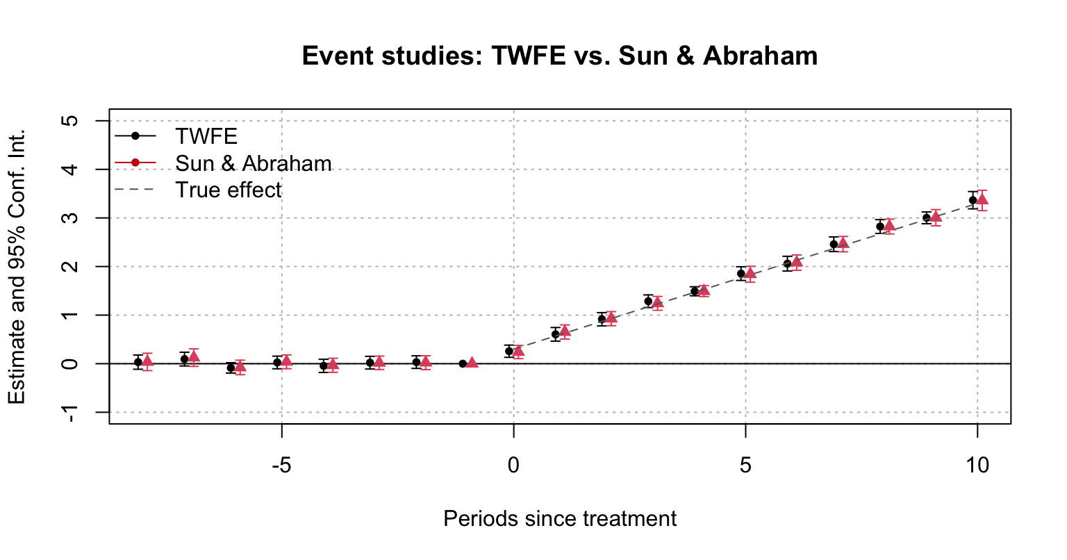
iplot(list(m_es_twfe, m_sa), xlim = c(-8, 10), ylim = c(-1, 5),
      main = "Event studies: TWFE vs. Sun & Abraham",
      xlab = "Periods since treatment")
lines(0:10, 0.3 * (0:10 + 1), lty = 2, col = "grey40")
legend("topleft", c("TWFE", "Sun & Abraham", "True effect"),
       col = c("black", "#CC0000", "grey40"), lty = c(1, 1, 2), pch = c(20, 20, NA), bty = "n")

Reading the Plot

Both event studies track the true dynamic effect here, because each period since treatment gets its own coefficient, every cohort follows the same dynamic path, and never-treated units give clean comparisons. The problem is the single static coefficient, which averages these growing effects using already-treated units as controls. A TWFE event study is not safe in general: when the dynamic path differs across cohorts, or when periods are binned or dropped, each coefficient can mix in effects from other periods, and spurious pre-trends can appear (Sun and Abraham 2021).

Real Data

Real Data: Minimum Wages and Teen Employment

Code

suppressMessages(library(did))
data(mpdta)   # 500 US counties, 2003-2007; some states raised their minimum wage in 2004, 2006, or 2007
mpdta$treated_now <- as.integer(mpdta$first.treat > 0 & mpdta$year >= mpdta$first.treat)

# Static TWFE vs. Callaway & Sant'Anna (2021), which only compares with not-yet- or never-treated counties
twfe <- feols(lemp ~ treated_now | countyreal + year, data = mpdta, cluster = ~countyreal)
set.seed(2026)
cs <- att_gt(yname = "lemp", tname = "year", idname = "countyreal", gname = "first.treat", data = mpdta)

round(c(TWFE = unname(coef(twfe)), Callaway_SantAnna = aggte(cs, type = "simple")$overall.att), 3)

             TWFE Callaway_SantAnna 
           -0.037            -0.040

mpdta ships with the did package: log teen employment by county, a subset of the data in Callaway & Sant’Anna (2021). Treated counties are in states that raised the minimum wage; controls are counties at the federal minimum throughout.
The two estimates are close here (about −4% teen employment), so TWFE does little harm. That is a finding, not a guarantee: always check.

Real Data: The Event Study

Code

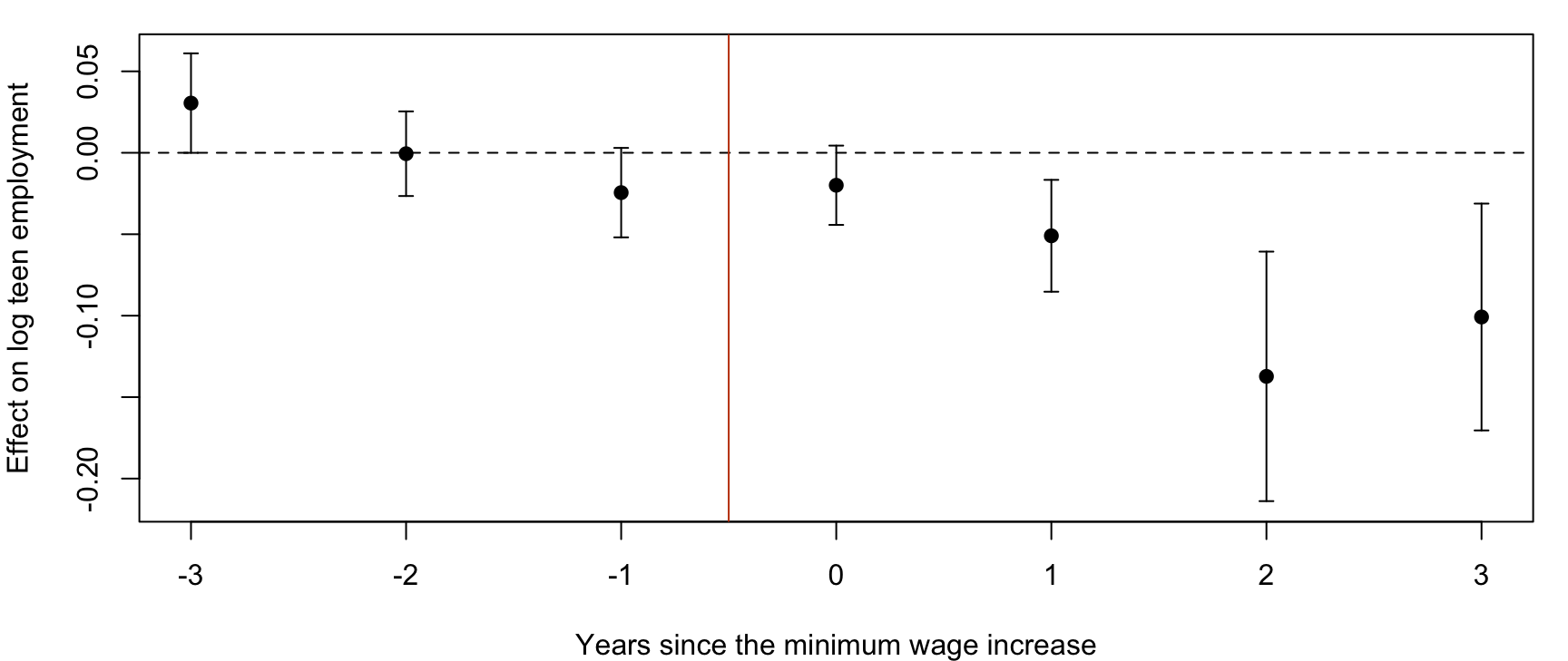
es <- aggte(cs, type = "dynamic")
par(mar = c(4, 4, 1, 1))
plot(es$egt, es$att.egt, pch = 19, ylim = range(es$att.egt - 2 * es$se.egt, es$att.egt + 2 * es$se.egt),
     xlab = "Years since the minimum wage increase", ylab = "Effect on log teen employment")
arrows(es$egt, es$att.egt - 1.96 * es$se.egt, es$egt, es$att.egt + 1.96 * es$se.egt, angle = 90, code = 3, length = 0.04)
abline(h = 0, lty = 2); abline(v = -0.5, col = "#c2410c")

Reading the Result

The effect grows with time since the increase. Before the increase, the estimates are close to zero but not perfectly flat, which is when the power of the pre-trend test and a sensitivity analysis (Rambachan and Roth 2023) matter.

Case Studies

Three Case Studies at a Glance

	Miller, Johnson & Wherry (2021)	Brynjolfsson, Li & Raymond (2025)	Demirci, Hannane & Zhu (2025)
Journal	Quarterly Journal of Economics	Quarterly Journal of Economics	Management Science
Question	Does Medicaid expansion reduce mortality?	Does a generative AI assistant raise worker productivity?	Which freelance jobs does generative AI replace?
Treated	Low-income adults in expansion states	Customer-support agents given the AI tool	Automation-prone job categories (writing, coding)
Control	Same group in non-expansion states	Agents not yet or never given the tool	Manual-intensive job categories
Timing	Staggered by state (2014–2017)	Staggered by agent (2020–2021)	One date: ChatGPT release (Nov 2022)
Robust estimator	Sun & Abraham (2021); Goodman-Bacon (2021) decomposition	Sun & Abraham; CS; dCDH; BJS	Callaway & Sant’Anna (2021); synthetic DiD

Keep asking the same three questions for each paper: (1) Who is the control group, and why is it a credible counterfactual? (2) What could break parallel trends? (3) How did the authors check?

Case Study 1: Medicaid and Mortality

Miller, Johnson & Wherry (2021), QJE (Miller et al. 2021)

Question: Did the ACA Medicaid expansions reduce mortality among low-income adults?

Data: a linkage of three federal sources:

American Community Survey (2008–2013) to identify people likely to gain eligibility: income at or below 138% of the poverty line or less than high school education; citizens; not already on disability benefits
Medicaid enrollment records to measure take-up
Census Numident death records to measure mortality through 2017

Sample: ~566,000 adults aged 55–64 in 2014 (a high-mortality group), excluding states that expanded before 2014.

Why it matters: earlier studies used aggregate death records and could not tell who was eligible, so they were underpowered to detect effects of plausible size.

Case Study 1: Specification

Event Study with Staggered State Adoption

Y_{isjt} = \text{Expansion}_s \times \sum_{\substack{y=-6 \\ y \neq -1}}^{3} \beta_y \,\mathbb{1}[t - t^*_s = y] + \beta_t + \beta_s + \beta_j + \gamma\,\mathbb{1}[j = t] + \varepsilon_{isjt}

Y: died during year t (linear probability model); individual i, state s, survey wave j
\beta_s state FE, \beta_t year FE, \beta_j survey-wave FE
t^*_s: the state’s expansion year (21 states in 2014; 6 later)
\beta_y for y < -1: pre-trend checks; y \geq 0: effects in each year after expansion
Standard errors clustered by state; ACS survey weights

A subtle point: the sample is a fixed cohort that ages, so mortality rises over time everywhere. The pre-period mean is the wrong baseline; the authors compute a counterfactual post-period mortality rate instead.

Case Study 1: Checking the Design

Checks the Authors Ran

First stage: Medicaid eligibility rises 49–51 pp and enrollment rises 12.8 pp in expansion states; flat beforehand.

Pre-trends: mortality trends are parallel before 2014. The authors then ask whether the test had power (Roth 2022): they could detect a linear pre-trend of 0.032 pp per year with 80% power; even such a trend would bias the estimate for event year 3 (the fourth year of expansion) by at most 0.089 pp, under half the estimated effect (0.208 pp).

Staggered timing: Goodman-Bacon (2021) decomposition shows only 11% of the TWFE weight comes from comparisons between differently timed states; dropping late expanders and using Sun & Abraham (2021) give similar results.

Placebo groups: no effect for people 65+ (already on Medicare), and only small effects for higher-income people, who were less likely to gain coverage.

Placebo period: no relative change in the pre-ACA period.

Other confounders: results are stable when adding state-specific linear trends, county economic trends, or alternative comparison groups.

Case Study 1: Results

Main Findings

Mortality falls by 0.132 percentage points per year, a 9.4% reduction relative to the sample mean
The effect grows over time: 0.089 pp in year 1, 0.208 pp by year 4
Driven by disease-related and health care–amenable deaths, not external causes such as accidents
Scaling: if non-expansion states had expanded, roughly 15,600 deaths could have been averted

From Intent-to-Treat to the Effect of Coverage

The DiD estimate is an intent-to-treat effect of living in an expansion state. Dividing by the first stage gives the effect of Medicaid itself, the same logic as IV in Chapters 5–6:

\frac{\text{reduced form}}{\text{first stage}} = \frac{0.132 \text{ pp}}{0.375 \text{ years of Medicaid}} \approx 0.35 \text{ pp lower mortality per year of coverage}

This scaled effect is a LATE for compliers: people who enrolled because of the expansion.

Case Study 1: What to Copy

Practices to Reuse

Define the exposed group precisely. Linked records identify people likely to gain eligibility, instead of diluting the effect over everyone.
Report the power of the pre-trend test: the trend they could have missed would bias the estimate by at most 0.089 pp.
Use a group that should not respond (people aged 65+, already on Medicare) as a placebo, and scale the ITT by the first stage.

Case Study 1: Discussion Questions

States chose whether to expand. Why doesn’t this choice by itself invalidate the design? What kind of state-level choice would?
Why is the elderly (65+) sample a useful placebo? What would a significant effect in that group have suggested?
The pre-trend test “passes”. Why do the authors still compute the size of trend they could have missed?
Only 11% of the TWFE weight comes from timing comparisons. Why does that make staggered-adoption bias a small concern here, but potentially a large one in other settings?
Why is the scaled effect (0.35 pp per year of coverage) a LATE, and for whom?

Case Study 2: Generative AI at Work

Brynjolfsson, Li & Raymond (2025), QJE (Brynjolfsson et al. 2025)

Question: Does a generative AI assistant raise the productivity of customer-support workers, and who benefits most?

Setting: a Fortune 500 software firm’s customer support. An AI tool built on GPT-3 reads live chats and suggests responses; agents can accept, edit, or ignore suggestions.

Data: 3 million chats by 5,172 agents (89% outside the US, mainly the Philippines), aggregated to agent × month.

Main outcome: resolutions per hour (issues successfully resolved per hour).

Why DiD: the tool was not given to everyone at once. Access was rolled out agent by agent between fall 2020 and early 2021.

Case Study 2: Where the Variation Comes From

Rollout Was Not Random. Is It Good Enough?

Constraints that created staggered timing:

Agents had to complete a 3-hour training session, run by only two trainers with limited weekly capacity
The firm had a fixed contractual budget for AI seats
Managers spread a team’s members across different sessions to avoid service disruption

The worry: managers chose who to onboard. Ever-treated agents were already better before AI access (2.0 vs. 1.7 resolutions per hour).

Why the design can still work: agent fixed effects absorb level differences. The threat is selection on trends: managers picking agents who were about to improve anyway.

Case Study 2: Specification and Checks

TWFE with Agent and Time Fixed Effects

y_{it} = \delta_t + \alpha_i + \beta \,AI_{it} + \gamma X_{it} + \varepsilon_{it}

\alpha_i agent FE; \delta_t year-month FE; X_{it} tenure FE (months on the job, since agents improve with experience)
AI_{it} = 1 once agent i has access; standard errors clustered by agent

Robustness:

Event study with the Sun & Abraham (2021) estimator: flat before access, immediate jump after
Similar results with Callaway & Sant’Anna (2021), de Chaisemartin & D’Haultfœuille (2020), and Borusyak, Jaravel & Spiess (2024) estimators
IV: instrument each agent’s adoption date with the date the first person in their team got access (rules out within-team selection by managers)
A small earlier RCT pilot (~50 workers) gives similar effects

Case Study 2: Results

Main Findings

Specification (resolutions per hour)	Estimate	Fixed effects
Time + location FE	+0.47 (+24%)	Year-month, location
+ Agent FE	+0.37	+ agent
+ Tenure FE (preferred)	+0.30 (+15%)	+ months of tenure

Adding agent FE shrinks the estimate: part of the raw gap was selection of stronger agents, which is what unit FE are for (Chapter 8).

Who gains: least-skilled and newest agents improve ~30%; the most skilled gain little, with a small decline in quality
Learning: agents with two months of tenure and AI perform like agents with six or more months without it; productivity stays higher even during AI outages
Work experience: customers are more polite and less likely to ask for a manager; attrition of new agents falls

Case Study 2: What to Copy

Practices to Reuse

Document how timing arose (trainer capacity, seat budgets) to argue it is unrelated to workers’ trends.
Report several heterogeneity-robust estimators next to TWFE.
Add a different design for the same question: a team-level instrument and a small randomized pilot.

Case Study 2: Discussion Questions

Ever-treated agents were more productive before AI. Why is this a problem for a cross-sectional comparison but not, by itself, for DiD with agent FE?
Why include tenure fixed effects in addition to agent and month FE? What bias would remain without them?
Why does instrumenting with the team’s first adoption date address manager selection? What does it assume?
The paper studies one firm in the medium run. What does it not tell us about generative AI’s effect on employment or wages?
The most-skilled agents follow AI suggestions more over time, even though quality falls slightly. Connect this to the idea of “cognitive surrender” (Chapter 4).

Case Study 3: Who Is AI Replacing?

Demirci, Hannane & Zhu (2025), Management Science (Demirci et al. 2025)

Question: How did ChatGPT (and image-generating AI) change demand for freelance work, and for which kinds of jobs?

Data: all job posts on a leading global freelancing platform, 2021–mid-2023: 1.2 million fixed-price posts from 542,000 employers in 61 countries.

Treated and control groups: job posts are clustered by skill tags into categories, then grouped by exposure to language models:

Treated (automation-prone): writing; software, app and web development; engineering
Control (manual-intensive): data and office management, video services, audio services
A separate analysis treats graphic design and 3D modeling as exposed to image-generating AI (Midjourney, DALL-E 2, Stable Diffusion)

Case Study 3: Specification

DiD with a Single, Common Shock

y_{ctl} = \beta \,(\text{Post}_t \times T_c) + \gamma_{cl} + \gamma_t + \varepsilon_{ctl}

y: log number of job posts in category c, week t, country l
\text{Post}_t: after ChatGPT’s release (30 November 2022); T_c: automation-prone category
\gamma_{cl} category × country FE; \gamma_t week FE (seasonality, platform trends)
Event-study version by month to check pre-trends
Standard errors clustered by job category

Note: everyone is “treated” on the same date, so there is no staggered-adoption problem. The authors still report Callaway & Sant’Anna (2021) and synthetic DiD estimates, plus a negative binomial model because log counts with zeros are problematic (Chen and Roth 2024).

Case Study 3: Results and Checks

Main Findings

Job posts in automation-prone categories fall 21% relative to manual-intensive ones within eight months (coefficient −0.234 on log posts)
By category: writing −30%, software/app/web development −21%, engineering −10%
Image-generating AI: graphic design and 3D modeling posts fall 17%
The effect grows over time and after more capable model releases
Remaining automation-prone jobs pay more (+5.7% maximum budget), are more complex (+2.2% skill tags), and attract more bids (+8.6%)

Strengthening the Causal Story

Dose-response: categories with larger increases in Google searches for “ChatGPT + [category]” saw larger declines
Placebo release dates give no effect
Robust to alternative control groups and to aggregating to category × week

Case Study 3: What to Copy

Practices to Reuse

When a shock hits everyone at once, compare exposed with unexposed categories, and argue that the controls are not exposed.
Add dose-response evidence (search intensity by category) and placebo release dates.
Pick a model that suits counts with zeros and be open about having few clusters.

Case Study 3: Discussion Questions

The “treatment” is a worldwide technology release on one date. Why is a comparison across job categories still needed? What would a simple before–after comparison of writing jobs pick up?
Could ChatGPT also affect the control categories (e.g., freelancers switching from writing to video editing, or clients using ChatGPT to write video scripts)? Which direction would that bias \hat\beta?
Standard errors are clustered by job category, with only a handful of categories. What inference concern does that raise, and what would you do about it?
Why might log(job posts) be a problematic outcome, and why does a negative binomial model help?
Compare with Case Study 2: one paper finds AI raises worker productivity, the other finds AI reduces demand for freelancers. Can both be true?

Comparing the Three Designs

	Miller et al. (2021)	Brynjolfsson et al. (2025)	Demirci et al. (2025)
Who chose treatment?	States (politics)	Managers and trainers	Nobody (technology release)
Main threat	State-level shocks around 2014	Selection of improving agents	Spillovers to control jobs
Key defence	Placebo groups, power analysis	Agent + tenure FE, team-level IV, RCT pilot	Dose-response via search data, placebo dates
Staggered timing?	Yes, mild	Yes, strong	No
Inference concern	46 state clusters	None (many agents)	Few category clusters

Best Practices

DiD Checklist

Before Estimating

Plot the raw data: treated and control group means over time
Justify the control group: why is its change a credible counterfactual?
Ask who chose treatment and why: selection on levels is fine; selection on trends is not
Choose the outcome scale (levels vs. logs) before looking at results
Decide the clustering level from how treatment was assigned

After Estimating

Show an event study and discuss the power of pre-trend tests
With staggered timing, report a heterogeneity-robust estimator alongside TWFE
Run placebo tests: unaffected groups, fake treatment dates
Check for spillovers onto the control group
Interpret the estimand: ATT for whom, over what horizon; scale by the first stage if treatment take-up is incomplete

Common Pitfalls

Mistakes to Avoid

Treating flat pre-trends as proof of parallel trends
Running static TWFE with staggered adoption and dynamic effects
Using already-treated units as controls without realizing it
Clustering too finely (by individual when the policy varies by state)
Controlling for post-treatment variables that the policy itself changes
Ignoring anticipation: units changing behaviour before the official start date
Ignoring spillovers: the control group is partly treated
Taking logs of outcomes with many zeros without thinking about what the estimate means

Summary

Key Ideas:

DiD compares changes, not levels: the control group’s change stands in for the treated group’s counterfactual change
Identification rests on parallel trends, plus no anticipation and no spillovers
DiD is the two-way fixed effects model from Chapter 8 with a policy that switches on at a known date

Summary: Modern Practice and Case Studies

Modern Practice:

Event studies show dynamics and pre-trends, but pre-trend tests have limited power
With staggered adoption, TWFE can mix in forbidden comparisons; use robust estimators
Cluster at the policy level; beware of few clusters

From the Case Studies:

Linked administrative data plus careful placebo tests make the Medicaid–mortality result credible
Generative AI raises productivity most for less experienced workers inside a firm…
…while reducing demand for automation-prone freelance work across a platform

Next Steps

Read: Miller et al. (2021) Sections IV–VI; Brynjolfsson et al. (2025) Sections IV–V
Practice: In the staggered simulation, make the effect constant and re-run. When does TWFE work?
Assignment: Write a one-page referee report on Demirci et al. (2025) focusing on the control group and inference
Next Class: Synthetic control, for when there is only one treated unit and no single good control group

References

Arkhangelsky, Dmitry, Susan Athey, David A Hirshberg, Guido W Imbens, and Stefan Wager. 2021. “Synthetic Difference-in-Differences.” American Economic Review 111 (12): 4088–118. https://doi.org/10.1257/aer.20190159.

Bertrand, Marianne, Esther Duflo, and Sendhil Mullainathan. 2004. “How Much Should We Trust Differences-in-Differences Estimates?” The Quarterly Journal of Economics 119 (1): 249–75.

Borusyak, Kirill, Xavier Jaravel, and Jann Spiess. 2024. “Revisiting Event-Study Designs: Robust and Efficient Estimation.” Review of Economic Studies 91 (6): 3253–85. https://doi.org/10.1093/restud/rdae007.

Brynjolfsson, Erik, Danielle Li, and Lindsey Raymond. 2025. “Generative AI at Work.” The Quarterly Journal of Economics 140 (2): 889–942. https://doi.org/10.1093/qje/qjae044.

Callaway, Brantly, and Pedro H C Sant’Anna. 2021. “Difference-in-Differences with Multiple Time Periods.” Journal of Econometrics 225 (2): 200–230. https://doi.org/10.1016/j.jeconom.2020.12.001.

Chaisemartin, Clément de, and Xavier D’Haultfœuille. 2020. “Two-Way Fixed Effects Estimators with Heterogeneous Treatment Effects.” American Economic Review 110 (9): 2964–96. https://doi.org/10.1257/aer.20181169.

Chen, Jiafeng, and Jonathan Roth. 2024. “Logs with Zeros? Some Problems and Solutions.” The Quarterly Journal of Economics 139 (2): 891–936. https://doi.org/10.1093/qje/qjad054.

Demirci, Ozge, Jonas Hannane, and Xinrong Zhu. 2025. “Who Is AI Replacing? The Impact of Generative AI on Online Freelancing Platforms.” Management Science 71 (10): 8097–108. https://doi.org/10.1287/mnsc.2024.05420.

Goodman-Bacon, Andrew. 2021. “Difference-in-Differences with Variation in Treatment Timing.” Journal of Econometrics 225 (2): 254–77.

Miller, Sarah, Norman Johnson, and Laura R Wherry. 2021. “Medicaid and Mortality: New Evidence from Linked Survey and Administrative Data.” The Quarterly Journal of Economics 136 (3): 1783–829. https://doi.org/10.1093/qje/qjab004.

Rambachan, Ashesh, and Jonathan Roth. 2023. “A More Credible Approach to Parallel Trends.” Review of Economic Studies 90 (5): 2555–91. https://doi.org/10.1093/restud/rdad018.

Roth, Jonathan. 2022. “Pretest with Caution: Event-Study Estimates After Testing for Parallel Trends.” American Economic Review: Insights 4 (3): 305–22. https://doi.org/10.1257/aeri.20210236.

Roth, Jonathan, and Pedro H C Sant’Anna. 2023. “When Is Parallel Trends Sensitive to Functional Form?” Econometrica 91 (2): 737–47. https://doi.org/10.3982/ECTA19402.

Sun, Liyang, and Sarah Abraham. 2021. “Estimating Dynamic Treatment Effects in Event Studies with Heterogeneous Treatment Effects.” Journal of Econometrics 225 (2): 175–99. https://doi.org/10.1016/j.jeconom.2020.09.006.